Versions of the library
Currently, the library consists of one major part, labelled ChASE-MPI, for solving dense eigenproblems. There will be another major part to support sparse eigenproblems in short future. ChASE-MPI can be installed with the minimum amount of dependencies (BLAS, LAPACK, and MPI).
ChASE-MPI
Multi-Configurations
ChASE-MPI supports different configurations depending on the available hardware resources.
Shared memory build: This is the simplest configuration and should be exclusively selected when ChASE is used on only one computing node or on a single CPU. The simplicity of this configuration resides in the way the Matrix-Matrix kernel is implemented with respect to the full MPI build.
MPI+Threads build: On multi-core homogeneous CPU clusters ChASE is best used in its pure MPI build. In this configuration, ChASE is typically used with one MPI rank per NUMA domain and as many threads as number of available cores per NUMA domain.
GPU build: ChASE-MPI can be configured to take advantage of graphics card on heterogeneous computing clusters. Currently we support one GPU card per MPI rank.
Matrix Distributions
In ChASE-MPI, the MPI nodes are constructed as 2D grid, two data distributions are support to assigned sub-blocks of dense matrix A into different MPI nodes.
Block Distribution
The first is called Block Distribution, in which each MPI rank of 2D grid is assigned a block of dense matrix A. The most important kernel of ChASE is the Hermitian Matrix-Matrix Multiplication. This block data distribution results in a matrix-matrix multiplications on each node that is large and contiguous, often resulting in a performance close to the hardware theoretical peak. In addition, this data distribution allows an easy offloading of the multiplication to accelerators such as GPUs.
The figure above gives an example of ChASE which distributes a \(n \times n\) dense matrix \(A\) into a \(3 \times 3\) grid of MPI nodes. In this example, the matrix A is split into 2D, with a series of sub-matrices \(A_{i,j}\) in which \(i \in [0,2]\) and \(j \in [0,2]\). Therefore, \(A_{0,0}\) is distributed to MPI rank 1, \(A_{1,0}\) is distributed to rank 2, \(A_{2,0}\) is distributed to rank 3, \(A_{0,1}\) is distributed to rank 4, \(A_{1,1}\) is distributed to rank 5, and so on.
Block-Cyclic Distribution
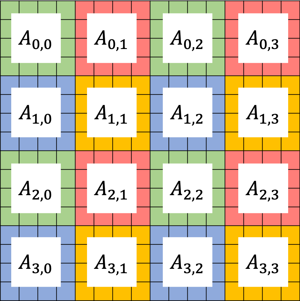
The second is called 2D Block-Cyclic Distribution. This distribution scheme was introduced for the implementation of dense matrix computations on distributed-memory machines. Compared to the Block Distribution, the main advantage of the Block-Cyclic Distribution is improving the load balance of matrix computation if the amount of work differs for different entries of a matrix, e.g., QR and LU factorization. A block distribution can lead to load imbalances.
Even the load balance is not a problem for ChASE, in which the most important kernel Hermitian Matrix-Matrix Multiplication is well balanced with the Block Distribution, we still provide the Block-Cyclic Distribution as an option in ChASE to avoid the re-distribution between these two types of distributions, which might be required for some application, e.g., solving generalized eigenproblem by ChASE with Cholesky factorization. In ChASE, its implementation with Block-Cyclic Distribution can achieve similar performance as the implementation with Block Distribution.

The figure above show an example of ChASE which distributes a \(n \times n\) dense matrix \(A\) into a \(2 \times 2\) grid of MPI nodes in a block-cyclic scheme. Denoting the 4 MPI nodes as \(P_{0,0}\), \(P_{0,1}\), \(P_{1,0}\), and \(P_{1,1}\), they are marked as green, red, blue and yellow, respectively on the figure above. In this example, the matrix A is split into 2D, with a series of sub-matrices \(A_{i,j}\) in which \(i \in [0,3]\) and \(j \in [0,3]\). Each sub-matrix is assigned to one MPI node in a round-robin manner so that each MPI rank gets several non-adjacent blocks. For more details about Block-Cyclic Distribution, please refer to Netlib website.